Custom search

Montag, 21. November 2016

Riverine landscape width of an alpine river from the source to the outlet ... an open attempt

The riverine landscape width of alpine rivers is permanently changing from the source to the outlet due to geomorphology and neighboring land use.

Let's try to get the riverine landscape width along the river course of the alpine river Inn running through the the federal state of Tyrol.

river Inn through the federal state of Tyrol; backgroud by basemap.at
Open ingredients:
Workflow:
  • extract the river Inn vector line from the river network by v.extract
  • calculate sample points e.g. every 10m along the river course by v.fixed.segmentpoints; the distance from source downstream is uploaded automatically to the attribute table
  • calculate transect lines right and left of the river e.g. every 10m along the river course by v.transects
  • upload the fitting distance from source downstream included in the sample points to the attribute table of the transect lines by v.distance
  • extract habitat map types typically for alpine rivers (e.g. alluvial forests, gravel bars, willow thickets, ...) from the habitat mapping vector data by v.extract
  • dissolve this extracted polygones by v.dissolve
  • clip the transect lines by the dissolved habitat vector map by v.overlay
  • upload the vector length of the clipped transect lines to the attribute table by v.to.db
  • export the clipped transect lines attribute table as a csv file by v.db.select
  • import the csv file into R and do some maths
Some preliminary results:

histogram of the riverine landscape width along the alpine river Inn in the federal state of Tyrol
kernel density plot of the riverine landscape width along the alpine river Inn in the federal state of Tyrol
riverine landscape width vs. distance from source downstream (km)
The riverine landscape width of the alpine river Inn seems to be quite uniform along the course within the federal state of Tyrol, with some increasing width downstream and maybe noisy artefacts.

Let's do some visual checks:

transects every 10m along the river course measuring the riverine landscape width; background basemap.at
The visual checks shows more or less the uniformity of the riverine landscape width along the river Inn in this area. 

Open data and open software may enable such analysis over a large area, though pre- and postprocessing cleaning steps are needed to reduce noise and artefacts.

Samstag, 30. Januar 2016

Alpine gravel-bed rivers ... seen from far above in the orbit

River ecosystems are connected on large spatial scales, have varied drivers, strong, and often conflicting, societal interests, and interacting management processes. Rivers and riverine landscapes are ecosystems significantly shaped by recurrent natural disturbances. These dynamic processes initiate a complex mosaic of  habitats resulting in a remarkable high diversity of aquatic, amphibious and terrestrial organisms linked

Alpine gravel-bed rivers are of European interest due to 2 directives: Habitats Directive and Water Framework Directive. Regarding Habitats Directive three typical habitats are listed and can be seen as a succession from highly dynamic (3220 Alpine rivers and the herbaceous vegetation along their banks) to medium dynamic (3230 Alpine rivers and their ligneous vegetation with Myricaria germanica) and moderately dynamic (3240 Alpine rivers and their ligneous vegetation with Salix elaeagnos) pioneer sites.

Let's have a look from the orbit at one of the last near natural alpine gravel-bed rivers in the Eastern Alps: Tagliamento.

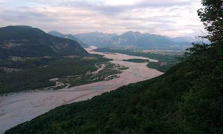
View to North from Monte Ragogna over Tagliamento's riverine landscape (photo: H. Kudrnovsky)
Ingedients:
Landsat 8 Operational Land Imager (OLI) and Thermal Infrared Sensor (TIRS) images consist of nine spectral bands with a spatial resolution of 30 meters for Bands 1 to 7 and 9. New band 1 (ultra-blue) is useful for coastal and aerosol studies. New band 9 is useful for cirrus cloud detection. The resolution for Band 8 (panchromatic) is 15 meters. Thermal bands 10 and 11 are useful in providing more accurate surface temperatures and are collected at 100 meters. Approximate scene size is 170 km north-south by 183 km east-west.

Landsat 8 data is available for download at no charge (e.g. Earth Explorer) and with no user restrictions.

First download Landsat 8 data and do a data check by gdalinfo:
Driver: GTiff/GeoTIFF
Files: LC81920282015221LGN00_B1.TIF
Size is 7651, 7771
Coordinate System is:
PROJCS["WGS 84 / UTM zone 32N",
    GEOGCS["WGS 84",
        DATUM["WGS_1984",
            SPHEROID["WGS 84",6378137,298.257223563,
                AUTHORITY["EPSG","7030"]],
            AUTHORITY["EPSG","6326"]],
        PRIMEM["Greenwich",0],
        UNIT["degree",0.0174532925199433],
        AUTHORITY["EPSG","4326"]],
    PROJECTION["Transverse_Mercator"],
    PARAMETER["latitude_of_origin",0],
    PARAMETER["central_meridian",9],
    PARAMETER["scale_factor",0.9996],
    PARAMETER["false_easting",500000],
    PARAMETER["false_northing",0],
    UNIT["metre",1,
        AUTHORITY["EPSG","9001"]],
    AUTHORITY["EPSG","32632"]]
Landsat 8 data is organized in UTM zones; here along the catchment of river Tagliamento UTM zone 32N. Import or link the data into a GRASS location created with EPSG: 32632 (UTM zone 32N).

Band 8 – Panchromatic (resolution 15m x 15m)
Let's have a look at the Landsat data within GRASS GIS:
i.landsat.toar -p input=LC81920282015221LGN00_B output=landsat_toar metfile=LC81920282015221LGN00_MTL.txt lsatmet=number,creation,date,sun_elev,sensor,bands,sunaz,time
number=8
creation=2015-08-09
date=2015-08-09
sun_elev=55.616710
sensor=OLI/TIRS
bands=11
sunaz=144.774232
The -p flag of the i.landsat.toar tool prints metadata info like sun azimuth, sun zenit (=elevation) and others.

Further i.landsat.toar is used to transform the calibrated digital number of Landsat imagery products to top-of-atmosphere radiance or top-of-atmosphere reflectance and temperature. Optionally, it can be used to calculate the at-surface radiance or reflectance with atmospheric correction (DOS method).  Atmospheric correction could also be done later by the dedicated i.atcorr tool.

Let's do the transformation with an atmospheric correction:
i.landsat.toar --verbose input=LC81920282015221LGN00_B output=dos1_corr_toar metfile=LC81920282015221LGN00_MTL.txt sensor=oli8 method=dos1
By i.colors.enhance an auto-balancing of colors for RGB images is performed.
i.colors.enhance red=dos1_corr_toar4 green=dos1_corr_toar3 blue=dos1_corr_toar2
RGB image (resolution 30m x 30m)
Habitat 3220 Alpine rivers and the herbaceous vegetation along their banks is typical for slightly vegetated gravel banks. Such sites often shows a high albedo. i.albedo computes broad band albedo from surface reflectance. In order to speed up computation time, e.g. the river (e.g. extracted from Natural Earth) can be buffered and a mask set by this buffer.
i.albedo -l -c --verbose input=dos1_corr_toar2,dos1_corr_toar3,dos1_corr_toar4,dos1_corr_toar5,dos1_corr_toar6,dos1_corr_toar7 output=tag_albedo_aggressivemode
i.albedo result; albedo raster values above a manually chosen threshold (here e.g. 0.19) clumped and vectorized
vectorized albedo above threshold 0.19 overlayed over a RGB image
The normalized difference vegetation index (NDVI) is a simple graphical indicator that can be used to analyze remote sensing measurements and assess whether the target being observed contains live green vegetation or not.
i.vi red=dos1_corr_toar4 output=vi_nvdi viname=nvdi nir=dos1_corr_toar5 green=dos1_corr_toar3 blue=dos1_corr_toar2 band5=dos1_corr_toar6t band7=dos1_corr_toar7
vectorized albedo above threshold 0.19 overlayed over a  NDVI map
vectorized albedo above threshold 0.19 overlayed over a panchromatic Landsat 8 image
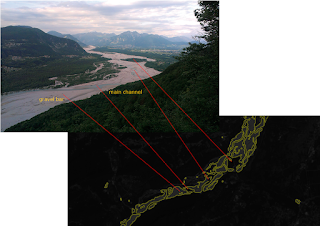
linking albedo analysis with nature

As the Landsat 8 satellite images the entire Earth every 16 days in an 8-day offset from Landsat 7, temporal and spatial analysis of alpine rivers and their gravel bed riverine landscape may be viable over large scale.

Combining available open source software (e.g. GRASS GIS, QGIS, Orfeo ToolBox) with open data (e.g. Landsat, Sentinel) tweaked by ground proofing may support to fulfill the targets of the EU directives (Habitats Directive, Water Framework Directive): sustainable water use and biodiversity preservation.

Donnerstag, 28. Januar 2016

Les Dolomites - an open GIS view on a World Heritage site

The United Nations Educational, Scientific and Cultural Organization (UNESCO) seeks to encourage the identification, protection and preservation of cultural and natural heritage around the world considered to be of outstanding value to humanity.

The Alpine Convention, an international treaty between the Alpine Countries (Austria, France, Germany, Italy, Liechtenstein, Monaco, Slovenia and Switzerland) as well as the EU for the sustainable development and protection of the Alps, had a working group UNESCO world heritage.

In June 2009 UNESCO listed the Dolomites as a World Heritage Site for the aesthetic value of its landscape and for the scientific importance of its geology and geomorphology.

Nine so called systems within the World Heritage Site:
  • Pelmo, Croda da Lago
  • Marmolada
  • Pale di San Martino, San Lucano, Dolomiti Bellunesi, Vette Feltrine
  • Dolomiti Friulane and d’Oltre Piave 
  • Dolomiti settentrionali 
  • Puez-Odle
  • Sciliar-Catinaccio, Latemar
  • Bletterbach
  • Dolomiti di Brenta
It's worth to visit them in nature!

The free and open pieces:
Download ASTER GDEM tiles freely from e.g. EarthExplorer and build a VRT from a list of the tiles by gdalbuildvrt.  
# GDAL
gdalbuildvrt asterv2.vrt -input_file_list aster_file_list.txt
Import the VRT into GRASS GIS.
 # GRASS GIS
r.in.gdal input=asterv2.vrt output=asterv2
Go to the ProtectedPlanet website and search for Italy to download the GIS data of italian protected areas; then search for Dolomites to get the related WDPA ID.
# GRASS GIS - import GIS data of  protected area with WDPA ID 478641 (Dolomites)
v.in.ogr input=WDPA_Jan2016_ITA-shapefile-polygons.shp layer=WDPA_Jan2016_ITA-shapefile-polygons output=world_heritage_site_les_dolomites where=WDPA_PID=478641
Import and reproject the Alpine Convention perimeter:
# GRASS GIS - reproject from EPSG 3035 while importing in a EPSG 4326 (WGS84) location
v.import input=AC-perimeter_ifuplan_16072007.shp output=world_heritage_site_les_dolomites epsg=3035
And then enjoy open data of a world heritage site and open GIS.
location of the world heritage site Dolomites within the perimeter of the Alpine Convention
ASTER GDEM of the southern Alps and world heritage site Dolomites
Smoothing the ASTER GDEM:
# GRASS GIS
r.neighbors input=asterv output=asterv2_rneigh_average_3x3 method=average size=3
ASTER GDEM and world heritage site Dolomites in 3D view (GRASS GIS) from southeast
ASTER GDEM and world heritage site Dolomites in 3D view (GRASS GIS) from southwest
As the Dolomites are known for their rich geomorphology, zoom in a bit.
ASTER GDEM and world heritage site Dolomites in 3D view (GRASS GIS) zoomed in
 ASTER GDEM and world heritage site Dolomites in a grey 3D view (GRASS GIS) zoomed in
ASTER GDEM and world heritage site Dolomites in 3D view (GRASS GIS) zoomed into slope map

Samstag, 21. November 2015

Forests of temperate Europe in the light of open data, open source software and SQL

According to the interpretation manual of the EU habitat directive some forests of community interest in the region of the temperate Europe are:
  • 9110 Luzulo-Fagetum beech forests 
  • 9120 Atlantic acidophilous beech forests with Ilex and sometimes also Taxus in the shrublayer (Quercinion robori-petraeae or Ilici-Fagenion)
  • 9130 Asperulo-Fagetum beech forests
  • 9140 Medio-European subalpine beech woods with Acer and Rumex arifolius
  • 9150 Medio-European limestone beech forests of the Cephalanthero-Fagion
  • 9160 Sub-Atlantic and medio-European oak or oakhornbeam forests of the Carpinion betuli
  • 9170 Galio-Carpinetum oak-hornbeam forests
  • 9180 * Tilio-Acerion forests of slopes, screes and ravines
  • 9190 Old acidophilous oak woods with Quercus robur on sandy plains
Some open ingredients for baking an analysis around these forests:
First download the spatialite version of the Natura 2000 data and have a quick look into the database by ogrinfo:
ogrinfo Natura2000_end2014.sqlite
INFO: Open of `Natura2000_end2014.sqlite'
      using driver `SQLite' successful.
1: natura2000polygon (Multi Polygon)
Beside the spatial data of protected areas within the Natura 2000 network (multipolygon layer: natura2000polygon), the database version of this data inlcudes also already additional informations connected to the protected areas (bioregion, contacts, designation status, directive species, habitat classes, habitats, impact, management, meta data, natura 2000 sites, other species, species).

Let's have a deeper look into the spatialite database (simplified by e.g. the spatialite-gui) and do some non-spatial SQL queries; e.g. filtering/querying the data and creating a view of protected areas including 9110 Luzulo-Fagetum beech forests:
# create view with protected areas including 9110 Luzulo-Fagetum beech forests based on the non-spatial table HABITATS
CREATE VIEW "vhabitat9110" AS
SELECT "SITECODE" AS "SITECODE", "HABITATCODE" AS "HABITATCODE",
    "COVER_HA" AS "COVER_HA", "REPRESENTATIVITY" AS "REPRESENTATIVITY",
    "RELSURFACE" AS "RELSURFACE", "CONSERVATION" AS "CONSERVATION",
    "GLOBAL_ASSESMENT" AS "GLOBAL_ASSESMENT", "DATAQUALITY" AS "DATAQUALITY",
    "PERCENTAGE_COVER" AS "PERCENTAGE_COVER"
FROM "HABITATS"
WHERE "HABITATCODE" = 9110
ORDER BY "SITECODE";
A view is some kind of a filtered/queried view of data organized like a table.

Just do it analogously for the other forest habitat types.

Then implement a spatial view of the data for later loading it to GIS:
# join the view created in the step before (vhabitat9110) with the spatial layer (Natura2000polygon) of the spatialite database.
CREATE VIEW "svhabitat9110" AS
SELECT "a"."ROWID" AS "ROWID", "a"."PK_UID" AS "PK_UID",
    "a"."SITECODE" AS "SITECODE", "a"."SITENAME" AS "SITENAME",
    "a"."RELEASE_DA" AS "RELEASE_DA", "a"."MS" AS "MS",
    "a"."SITETYPE" AS "SITETYPE", "a"."Geometry" AS "Geometry",
    "b"."SITECODE" AS "SITECODE_1", "b"."HABITATCODE" AS "HABITATCODE",
    "b"."COVER_HA" AS "COVER_HA", "b"."REPRESENTATIVITY" AS "REPRESENTATIVITY",
    "b"."RELSURFACE" AS "RELSURFACE", "b"."CONSERVATION" AS "CONSERVATION",
    "b"."GLOBAL_ASSESMENT" AS "GLOBAL_ASSESMENT", "b"."DATAQUALITY" AS "DATAQUALITY",
    "b"."PERCENTAGE_COVER" AS "PERCENTAGE_COVER"
FROM "Natura2000polygon" AS "a"
JOIN "vhabitat9110" AS "b" USING ("SITECODE")
ORDER BY "a"."SITECODE";

# registration of the spatial view to be loadable for GIS
INSERT INTO views_geometry_columns
    (view_name, view_geometry, view_rowid, f_table_name, f_geometry_column, read_only)
  VALUES ('svhabitat9110', 'geometry', 'rowid', 'natura2000polygon', 'geometry', 1);
A spatial view is some kind of a filtered/queried view of spatial data organized in a spatial database.

Do the same also for the other forest habitat types and have a look into the database:
ogrinfo Natura2000_end2014.sqlite
INFO: Open of `Natura2000_end2014.sqlite'
      using driver `SQLite' successful.
1: natura2000polygon (Multi Polygon)
2: svhabitat9110 (Multi Polygon)
3: svhabitat9120 (Multi Polygon)
4: svhabitat9130 (Multi Polygon)
5: svhabitat9140 (Multi Polygon)
6: svhabitat9150 (Multi Polygon)
7: svhabitat9160 (Multi Polygon)
8: svhabitat9170 (Multi Polygon)
9: svhabitat9180 (Multi Polygon)
10: svhabitat9190 (Multi Polygon)
Now there are spatial views of several forest habitat types.

Open QGIS, load the spatial views of protected areas with forest and let's do some further analysis, e.g. calculate the polygon centroids (in QGIS: Vector -> Geometry tools -> Polygon centroid) and a Delaunay triangulation of the centroids (in QGIS: Vector -> Geometry tools -> Delaunay triangulation) showing the function of an ecological network of protected areas for a certain habitat type in a simple way.

Some overviews of the distribution of some European temperate forest types within the Natura 2000 network by centroids of protected areas, connected by a Delaunay triangulation:

9110 Luzulo-Fagetum beech forests
9120 Atlantic acidophilous beech forests with Ilex and sometimes also Taxus in the shrublayer (Quercinion robori-petraeae or Ilici-Fagenion)
9130 Asperulo-Fagetum beech forests
9140 Medio-European subalpine beech woods with Acer and Rumex arifolius
9150 Medio-European limestone beech forests of the Cephalanthero-Fagion
9160 Sub-Atlantic and medio-European oak or oakhornbeam forests of the Carpinion betuli
9170 Galio-Carpinetum oak-hornbeam forests
9180 * Tilio-Acerion forests of slopes, screes and ravines
9190 Old acidophilous oak woods with Quercus robur on sandy plains
Another nice example of a interaction/interplay of open data and open source software to get an overview of European nature.


Mittwoch, 23. September 2015

biodiversity and red list spatial data along the open way

Biodiversity is declining worldwide. Red lists and available biodiversity data are the basics for conservation.

The IUCN, International Union for Conservation of Nature, provides Red List of Threatened Species with taxonomic, conservation status and distribution information on plants, fungi and animals that have been globally evaluated using the IUCN Red List Categories and Criteria.

GBIF provides free and open access to biodiversity data.

Let's see what you can do with these informations along the open way, e.g. on the example of Triturus carnifex:

"This species is sensitive to changes in water quality. The principal threats to the species are loss of aquatic habitats, especially breeding sites, through agricultural intensification and agrochemical pollution, and introduction of predatory fishes. In the Balkans, there has been loss of breeding habitats in recent years due to decreased spring rains, perhaps as a result of global climate change, and presumed mortality of individuals because of predation by introduced fishes." (IUCN 2015)

Open data
Open source software
Some commands in GRASS GIS to get an overview:
# link to Natural Earth Admin 0 - Countries
v.external input=C:\dl\iucn\ne_10m_admin_0_countries output=ne_10m_admin_0_countries layer=ne_10m_admin_0_countries

# import downloaded GBIF data of Triturus carnifex
v.in.gbif -c --verbose input=C:\dl\iucn\triturus\0000336-150922153815467.csv \ output=GBIF_Triturus_carnifex dir=C:\dl\iucn\triturus 

# import IUCN Red List Spatial Data defined filtered for Triturus carnifex
v.in.redlist input=C:\dl\iucn\CAUDATA\CAUDATA.shp output=IUCN_redlist_Triturus_carnifex \ species_name="Triturus carnifex"

Triturus carnifex: blue points (GBIF data), grey polygon (IUCN Red List Spatial data), red lines (Natural Earth Data)
These are nice basic data and tools to help improving biodiversity status. Let's contribute to extend!